【Class】CMU 10-414(714) Deep Learning Systems

课程

2022年课程视频 + 2025年PPT

课程视频

Lecture 1 - Introduction and Logistics

课程信息

Deep Learning Systems

Assignments

Assignments

Lecture 1: Introduction and Logistics

Elements of deep learning systems
Compose multiple tensor operations to build modern machine learning models
Transform a sequence of operations (automatic differentiation (微分))
Accelerate computation via specialized hardware
Extend more hardware backends, more operators

Lecture 2: ML Refresher / Softmax Regression

Basics of machine learning

Machine learning as data-driven programming
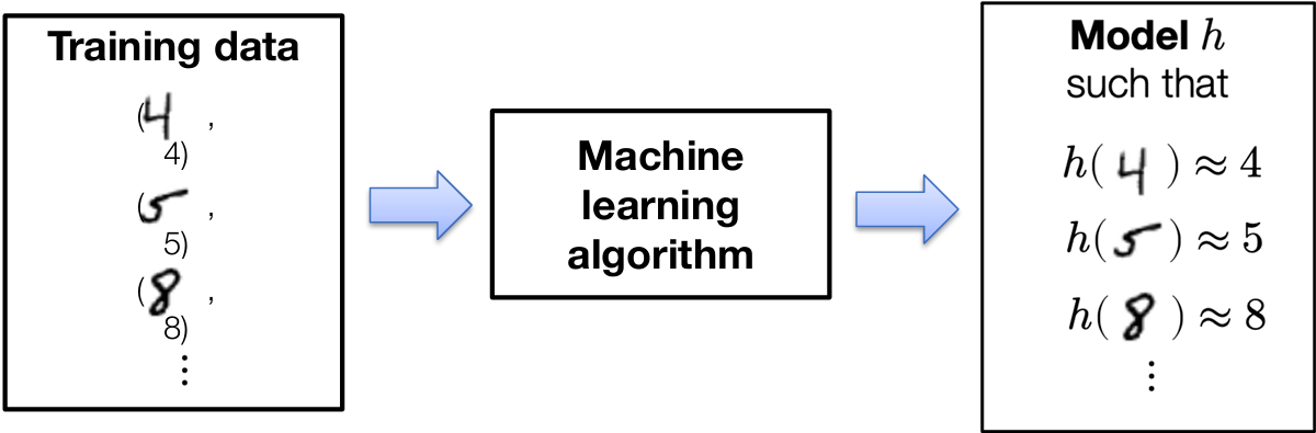
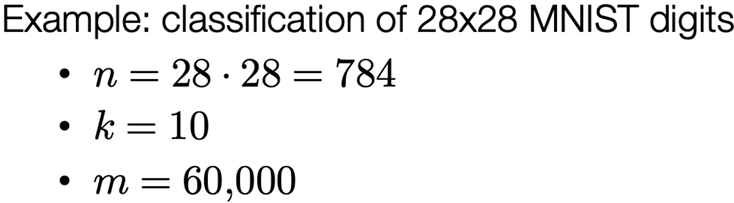
Suppose you want to write a program that will classify handwritten drawing of digits into their appropriate category: 0,1,…,9

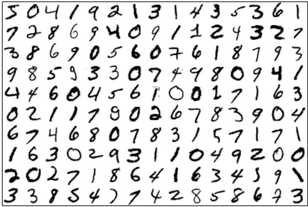
MNIST Dataset
The (supervised) ML approach: collect a training set of images with known labels and feed these into a machine learning algorithm, which will (if done well), automatically produce a “program” that solves this task

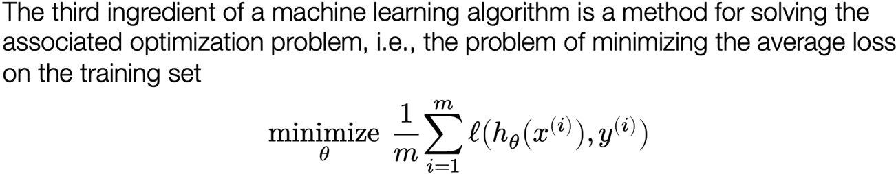
Three ingredients of a machine learning algorithm
Every machine learning algorithm consists of three different elements:
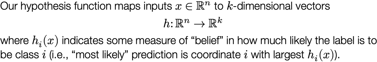
The hypothesis class: the “program structure”, parameterized via a set of parameters, that describes how we map inputs (e.g., images of digits) to outputs (e.g., class labels, or probabilities of different class labels)
The loss function: a function that specifies how “well” a given hypothesis (i.e., a choice of parameters) performs on the task of interest
An optimization method: a procedure for determining a set of parameters that (approximately) minimize the sum of losses over the training set

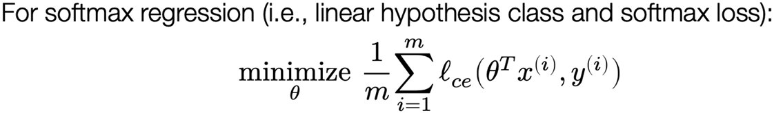
Example: softmax regression

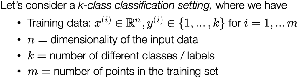
Multi-class classification setting

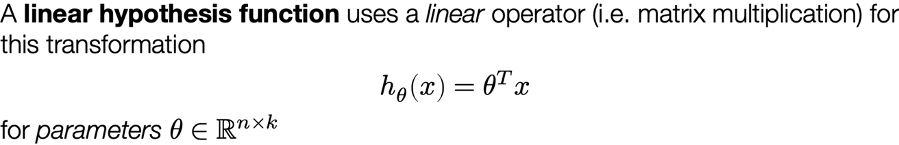
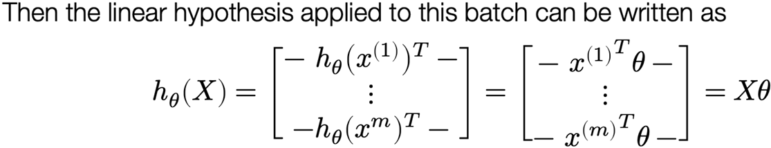
Linear hypothesis function

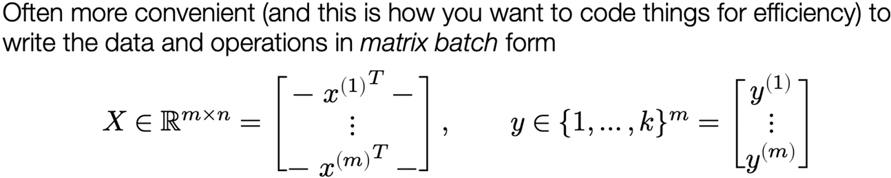
Matrix batch notation

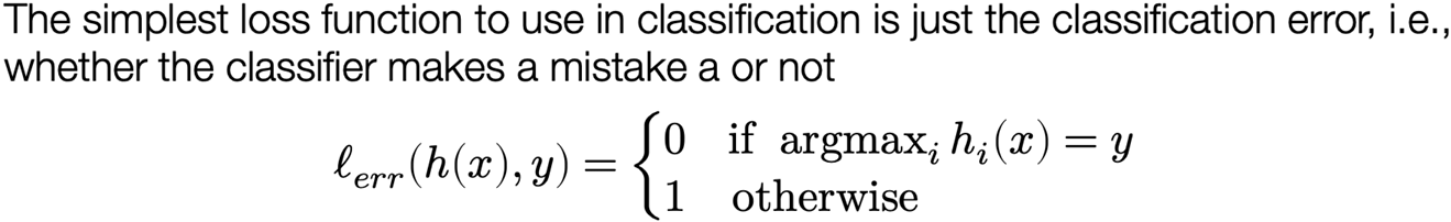
Loss function #1: classification error

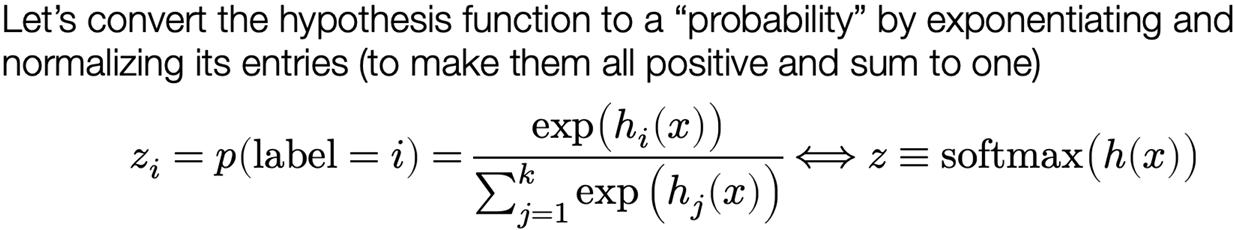
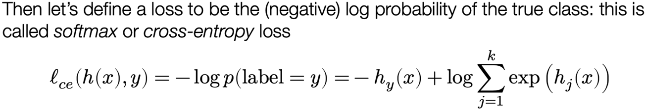
Loss function #2: softmax / cross-entropy loss

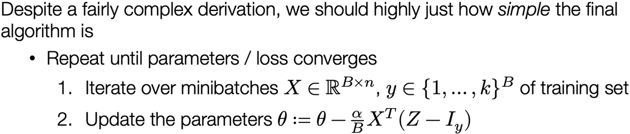
The softmax regression optimization problem

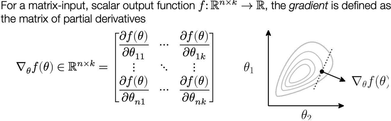
Optimization: gradient descent

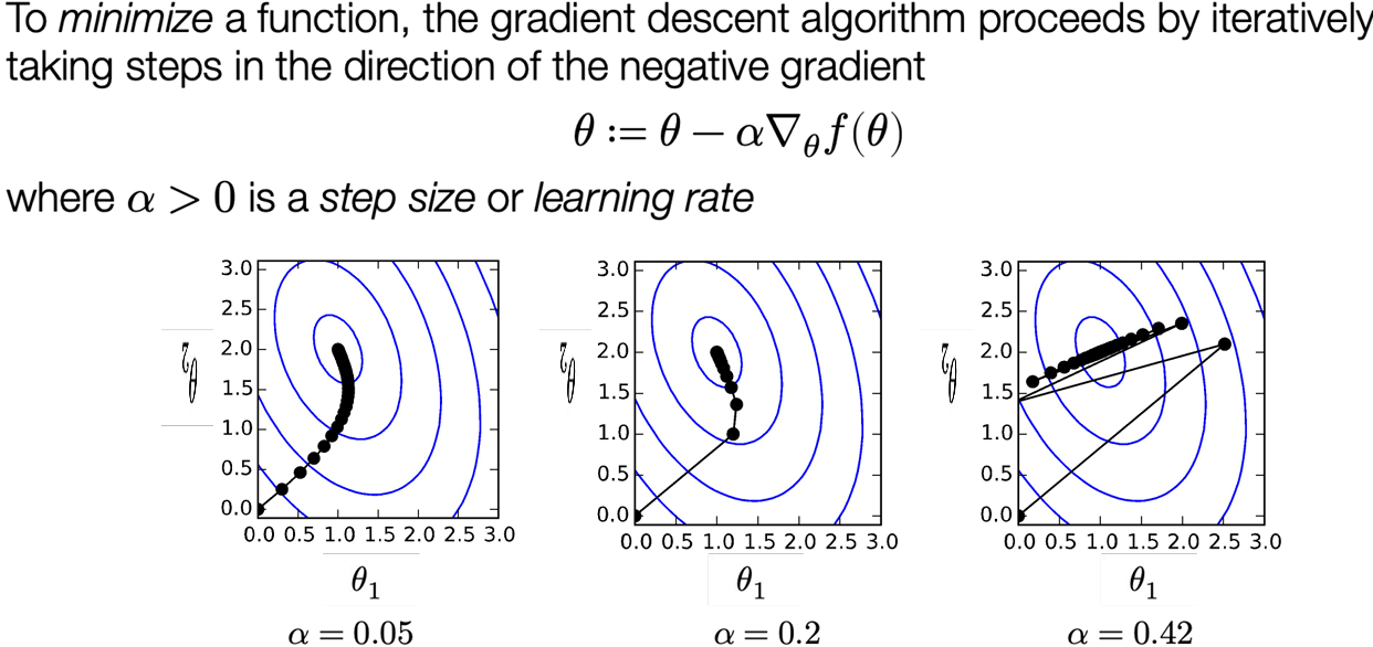
Stochastic gradient descent

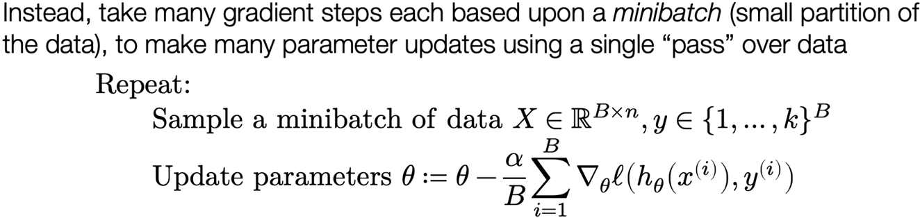
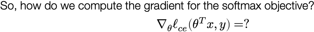
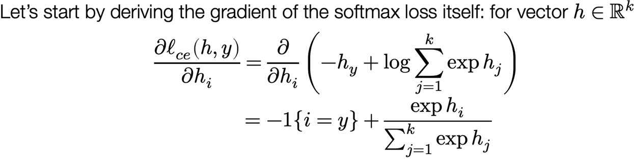
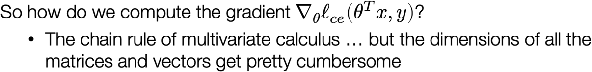
The gradient of the softmax objective

​
​
​

Putting it all together

Lecture 3: “Manual” Neural Networks

From linear to nonlinear hypothesis classes

The trouble with linear hypothesis classes

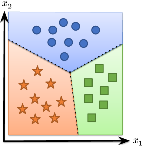
Recall that we needed a hypothesis function to map inputs in Rⁿ to outputs (class logits) in R^k, so we initially used the linear hypothesis class

This classifier essentially forms k linear functions of the input and then predicts the class with the largest value: equivalent to partitioning the input into k linear regions corresponding to each class

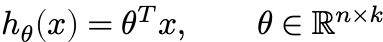
What about nonlinear classification boundaries?

What if we have data that cannot be separated by a set of linear regions?
We want some way to separate these points via a nonlinear set of class boundaries
One idea: apply a linear classifier to some (potentially higher-dimensional) features of the data
$$
h_\theta(x) = \theta^T \phi(x)\
\theta \in \mathbb{R}^{d \times k}, , \phi: \mathbb{R}^n \to \mathbb{R}^d
$$
How do we create features?
How can we create the feature function Φ?
1.Through manual engineering of features relevant to the problem (the “old” way of doing machine learning)
2.In a way that itself is learned from data (the “new” way of doing ML)
First take: what if we just again use a linear function for Φ?
$$
\phi(x) = W^T x
$$
​ Doesn’t work, because it is just equivalent to another linear classifier
$$
h_\theta(x) = \theta^T \phi(x) = \theta^T W^T x = \tilde{\theta} x
$$
Nonlinear features
But what does work? essentially any nonlinear function of linear features
$$
\phi(x) = \sigma(W^T x)
$$
​ where W ∈ R^{n x d}, and σ: R^d → R^d is essentially any nonlinear function
​ Example: let W be a (fixed) matrix of random Gaussian samples, and let σ be the cosine function ===> “random Fourier features” (work great for many problems)
​ But maybe we want to train W to minimize loss as well? Or maybe we want to compose multiple features together?

Neural networks

Neural networks / deep learning
A neural network refers to a particular type of hypothesis class, consisting of multiple, parameterized differentiable functions (a.k.a. “layers”) composed together in any manner to form the output
The term stems from biological inspiration, but at this point, literally any hypothesis function of the type above is referred to as a neural network
“Deep network” is just a synonym for “neural network,” and “deep learning” just means “machine learning using a neural network hypothesis class” (let’s cease pretending that there is any requirements on depth beyond “just not linear”)
But it’s also true that modern neural networks involve composing together a lot of functions, so “deep” is typically an appropriate qualifier

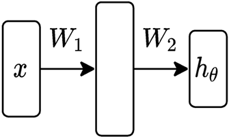
The “two layer” neural network
We can begin with the simplest form of neural network, basically just the nonlinear features proposed earlier, but where both sets of weights are learnable parameters
$$
h_\theta(x) = W_2^T \sigma(W_1^T x)\
\theta = {W_1 \in \mathbb{R}^{n \times d}, W_2 \in \mathbb{R}^{d \times k}}
$$
​ where σ: R → R is a nonlinear function applied elementwise to the vector (e.g. sigmoid, ReLU)
​ Written in batch matrix form
$$
h_\theta(X) = \sigma(XW_1)W_2
$$

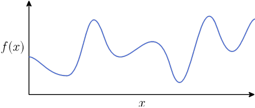
Universal function approximation
Theorem (1D case): Given any smooth function f: R → R, closed region D ⊂ R, and ε > 0, we can construct a one-hidden-layer neural network such that
$$
\max_{x \in D} |f(x) - \hat{f}(x)| \leq \epsilon
$$
​ Proof: Select some dense sampling of points (x⁽ⁱ⁾, f(x⁽ⁱ⁾)) over D. Create a neural network that passes exactly through these points. Because the neural network function is piecewise linear, and the function f is smooth, by choosing the x⁽ⁱ⁾ close enough together, we can approximate the function arbitrarily closely
​ Assume one-hidden-layer ReLU network (w / bias):
$$
\hat{f}(x) = \sum_{i=1}^d \pm \max{0, w_i x + b_i}
$$
​ Visual construction of approximating function
​

Fully-connected deep networks

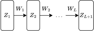
A more generic form of a L-layer neural network - a.k.a. “Multi-layer perceptron” (MLP), feedforward network, fully-connected network – (in batch form)
$$
Z_{i+1} = \sigma_i(Z_iW_i), , i = 1, …, L\
Z_1 = X,\
h_\theta(X) = Z_{L+1}\
[Z_i \in \mathbb{R}^{m \times n_i}, , W_i \in \mathbb{R}^{n_i \times n_{i+1}}]
$$
​ with nonlinearities σ_i: R → R applied elementwise, and parameters
$$
\theta = {W_1, \dots, W_L}
$$
​ (Can also optionally add bias term)

Why deep networks?
They work like the brain!
… no they don’t!
Deep circuits are provably more efficient!
… at representing functions neural networks cannot actually learn (e.g. parity)!
Empirically it seems like they work better for a fixed parameter count!
… okay!

Backpropagation (i.e., computiing gradients)

Neural networks in machine learning
Recall that neural networks just specify one of the “three” ingredients” of a machine learning algorithm, also need:
Loss function: still cross entropy loss, like last time
Optimization procedure: still SGD, like last time
In other words, we still want to solve the optimization problem
$$
\underset{\theta}{\text{minimize}} \quad \frac{1}{m} \sum_{i=1}^{m} \ell_{ce}(h_\theta(x^{(i)}), y^{(i)})
$$
​ using SGD, just with h_θ(x) now being a neural network
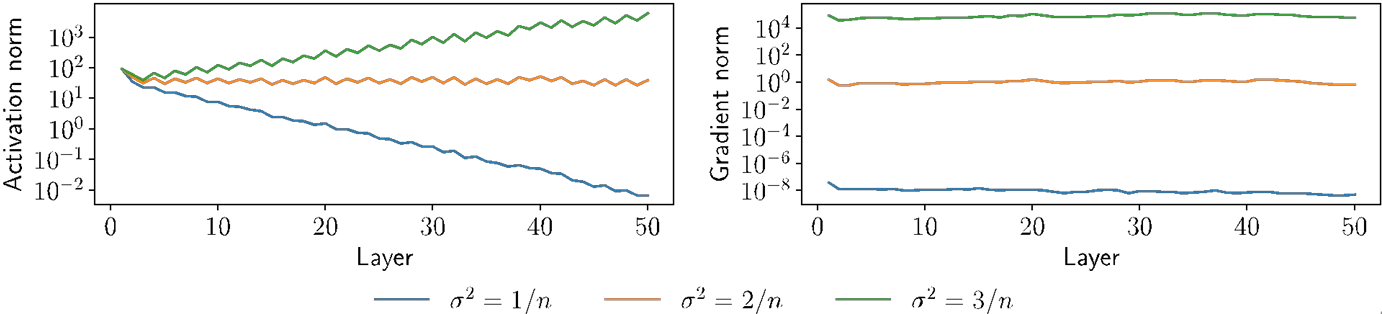
​ Requires computing the gradients 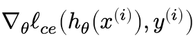for each element of θ

The gradient(s) of a two-layer network
Let’s work through the derivation of the gradients for a simple two-layer network, written in batch matrix form, i.e.,
$$ \nabla_{\{W_1, W_2\}} \ell_{ce}(\sigma(XW_1)W_2, y) $$ ​
​ The gradient w.r.t. W₂ looks identical to the softmax regression case:
$$
\frac{\partial \ell_{ce}(\sigma(XW_1)W_2, y)}{\partial W_2} = \frac{\partial \ell_{ce}(\sigma(XW_1)W_2, y) }{\partial \sigma(XW_1)W_2} \cdot \frac{\partial \sigma(XW_1)W_2}{\partial W_2} = (S - I_y) \cdot (\sigma(XW_1))\
[S = \text{normalize}(\exp(\sigma(XW_1)W_2))]
$$
​ so (matching sizes) the gradient is
$$
\nabla_{W_2} \ell_{ce}(\sigma(XW_1)W_2, y) = \sigma(XW_1)^T (S - I_y)
$$
​ Deep breath and let’s do the gradient w.r.t. W₁ …
$$
\frac{\partial \ell_{ce}(\sigma(XW_1)W_2, y)}{\partial W_1} = \frac{\partial \ell_{ce}(\sigma(XW_1)W_2, y)}{d\sigma(XW_1)W_2} \cdot \frac{d\sigma(XW_1)W_2}{d\sigma(XW_1)} \cdot \frac{d\sigma(XW_1)}{dXW_1} \cdot \frac{dXW_1}{dW_1}\
= (S - I_y) \cdot (W_2) \cdot (\sigma’(XW_1)) \cdot (X)
$$
​ and so the gradient is
$$
\nabla_{W_1} \ell_{ce}(\sigma(XW_1)W_2, y) = X^T \left( (S - I_y) W_2^T \circ \sigma’(XW_1) \right)
$$
​ wheredenotes elementwise multiplication
​ … having fun yet?

Backpropagation “in general”
There is a method to this madness … consider our fully-connected network:
$$
Z_{i+1} = \sigma_i(Z_iW_i), \quad i = 1, \dots, L
$$
​ Then (now being a bit terse with notation)
​
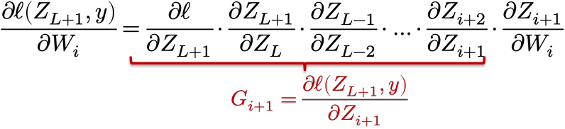
​ Then we have a simple “backward” iteration to compute the G_i‘s
$$
G_i = G_{i+1} \cdot \frac{\partial Z_{i+1}}{\partial Z_i} = G_{i+1} \cdot \frac{\partial \sigma_i(Z_i W_i)}{\partial Z_i W_i} \cdot \frac{\partial Z_i W_i}{\partial Z_i} = G_{i+1} \cdot \sigma’(Z_i W_i) \cdot W_i
$$
Computing the real gradients
To convert these quantities to “real” gradients, consider matrix sizes
$$
G_i = \frac{\partial \ell(Z_{L+1}, y)}{\partial Z_i} = \nabla_{Z_i} \ell(Z_{L+1}, y) \in \mathbb{R}^{m \times n_i}
$$
​ so with “real” matrix operations
$$
G_i = G_{i+1} \cdot \sigma’(Z_i W_i) \cdot W_i = (G_{i+1} \circ \sigma’(Z_i W_i))W_i^T
$$
​ Similar formula for actual parameter gradients
$$
\nabla_{W_i} \ell(Z_{L+1}, y) \in \mathbb{R}^{n_i \times n_{i+1}}
$$

$$
\frac{\partial \ell(Z_{L+1}, y)}{\partial W_i} = G_{i+1} \cdot \frac{\partial \sigma_i(Z_i W_i)}{\partial Z_i W_i} \cdot \frac{\partial Z_i W_i}{\partial W_i} = G_{i+1} \cdot \sigma’(Z_i W_i) \cdot Z_i\
\Rightarrow \nabla_{W_i} \ell(Z_{L+1}, y) = Z_i^T (G_{i+1} \circ \sigma’(Z_i W_i))
$$

Backpropagation: Forward and backward passes
Putting it all together, we can efficiently compute all the gradients we need for a neural network by following the procedure below

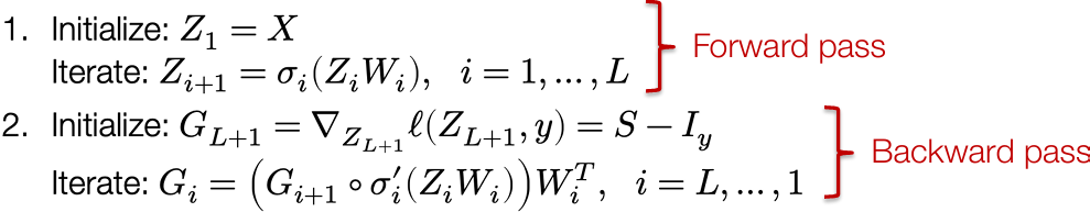
And we can compute all the needed gradients along the way
$$
\nabla_{W_i} \ell(Z_{k+1}, y) = Z_i^T \left( G_{i+1} \circ \sigma’_i(Z_i W_i) \right)
$$
​ “Backpropagation” is just chain rule + intelligent caching of intermediate results

A closer look at these operations
What is really happening with the backward iteration?

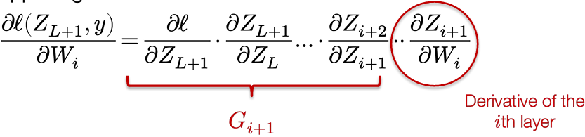
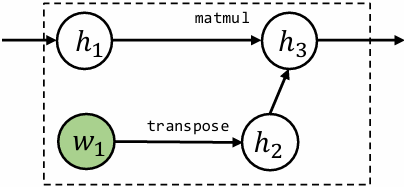
Each layer needs to be able to multiply the “incoming backward” gradient G_i+1 by its derivatives, , an operation called the “vector Jacobian product”
This process can be generalized to arbitrary computation graphs: this is exactly the process of automatic differentiation we will discuss in then next lecture

Homework 0

[WorldClass/CMU 10-414(714) Deep Learning Systems/Assignments/Homework 0 at master · tiny-star3/WorldClass](https://github.com/tiny-star3/WorldClass/tree/master/CMU 10-414(714) Deep Learning Systems/Assignments/Homework 0)

Lecture 4: Automatic Differentiation

General introduction to different differentiation methods

How does differentiation fit into machine learning
1.The hypothesis class:

2.The loss function:
$$
l(h_\theta(x), y) = -h_y(x) + \log \sum_{j=1}^k \exp(h_j(x))
$$
​ 3.An optimization method:
$$
\theta := \theta - \frac{\alpha}{B} \sum_{i=1}^{B} \left[ \nabla_{\theta} \ell(h_{\theta}(x^{(i)}), y^{(i)}) \right]
$$
​ Recap: every machine learning algorithm consists of three different elements
​ Computing the loss function gradient with respect to hypothesis class parameters is the most common operation in machine learning

Numerical differentiation
Directly compute the partial gradient by definition
$$
\frac{\partial f(\theta)}{\partial \theta_i} = \lim_{\epsilon \to 0} \frac{f(\theta + \epsilon e_i) - f(\theta)}{\epsilon}
$$
​ A more numerically accurate way to approximate the gradient
$$
\frac{\partial f(\theta)}{\partial \theta_i} = \frac{f(\theta + \epsilon e_i) - f(\theta - \epsilon e_i)}{2\epsilon} + o(\epsilon^2)
$$
​ Suffer from numerical error, less efficient to compute

Numerical gradient checking
However, numerical differentiation is a powerful tool to check an implement of an automatic differentiation algorithm in unit test cases
$$
\delta^T \nabla_\theta f(\theta) = \frac{f(\theta + \epsilon\delta) - f(\theta - \epsilon\delta)}{2\epsilon} + o(\epsilon^2)
$$
​ Pick 𝛿 from unit ball, check the above invariance

Symbolic differentiation
Write down the formulas, derive the gradient by sum, product and chain rules
$$
\frac{\partial(f(\theta)+g(\theta))}{\partial \theta} = \frac{\partial f(\theta)}{\partial \theta} + \frac{\partial g(\theta)}{\partial \theta}\
\frac{\partial(f(\theta)g(\theta))}{\partial \theta} = g(\theta)\frac{\partial f(\theta)}{\partial \theta} + f(\theta)\frac{\partial g(\theta)}{\partial \theta}\
\frac{\partial f(g(\theta))}{\partial \theta} = \frac{\partial f(g(\theta))}{\partial g(\theta)} \frac{\partial g(\theta)}{\partial \theta}
$$
​ Naively do so can result in wasted computations
​ Example:
$$
f(\theta) = \prod_{i=1}^{n} \theta_i\
\frac{\partial f(\theta)}{\partial \theta_k} = \prod_{j \neq k} \theta_j
$$
​ Cost 𝑛(𝑛 −2) multiplies to compute all partial gradients

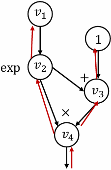
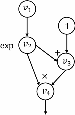
Computational graph
$$
y = f(x_1, x_2) = \ln(x_1) + x_1 x_2 - \sin x_2
$$
​
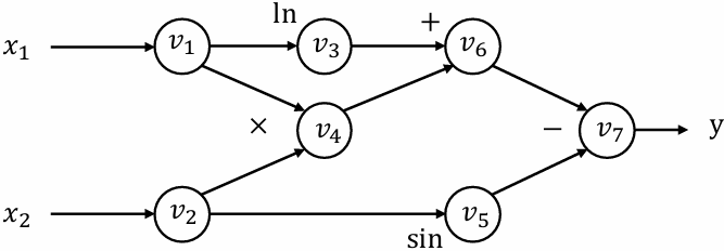
​ Forward evaluation trace
​ 𝑣₁ = 𝑥₁ = 2
​ 𝑣₂ = 𝑥₂ = 5
​ 𝑣₃ = ln𝑣₁ = ln2 = 0.693
​ 𝑣₄ = 𝑣₁ × 𝑣₂ = 10
​ 𝑣₅ = sin𝑣₂ = sin5 = −0.959
​ 𝑣₆ = 𝑣₃ + 𝑣₄ = 10.693
​ 𝑣₇ = 𝑣₆ − 𝑣₅ = 10.693 + 0.959 = 11.652
​ 𝑦 = 𝑣₇ = 11.652
​ Each node represent an (intermediate) value in the computation
​ Edges present input output relations

Forward mode automatic differentiation (AD)
Define
$$
\dot{v}_i = \frac{\partial v_i}{\partial x_1}
$$
​ We can then compute the iteratively in the forward topological order of the computational graph
​ Forward AD trace
$$
\begin{align*}
\dot{v}_1 &= 1 \
\dot{v}_2 &= 0 \
\dot{v}_3 &= \dot{v}_1 / v_1 = 0.5 \
\dot{v}_4 &= \dot{v}_1 v_2 + \dot{v}_2 v_1 = 1 \times 5 + 0 \times 2 = 5 \
\dot{v}_5 &= \dot{v}_2 \cos v_2 = 0 \times \cos 5 = 0 \
\dot{v}_6 &= \dot{v}_3 + \dot{v}_4 = 0.5 + 5 = 5.5 \
\dot{v}_7 &= \dot{v}_6 - \dot{v}_5 = 5.5 - 0 = 5.5
\end{align*}
$$
​ Now we have
$$
\frac{\partial y}{\partial x_1} = \dot{v}_7 = 5.5
$$
Limitation of forward mode AD
For 𝑓: ℝ^𝑛 → ℝ^𝑘, we need 𝑛 forward AD passes to get the gradient with respect to each input
We mostly care about the cases where 𝑘 = 1 and large 𝑛
In order to resolve the problem efficiently, we need to use another kind of AD

Reverse mode automatic differentiation

Reverse mode automatic differentiation(AD)
Define adjoint
$$
\overline{v}_i = \frac{\partial y}{\partial v_i}
$$
​ We can then compute the iteratively in the reverse topological order of the computational graph
​ Reverse AD evaluation trace
$$
\begin{align*}
\overline{v}_7 &= \frac{\partial y}{\partial v_7} = 1 \
\overline{v}_6 &= \overline{v}_7 \frac{\partial v_7}{\partial v_6} = \overline{v}_7 \times 1 = 1 \
\overline{v}_5 &= \overline{v}_7 \frac{\partial v_7}{\partial v_5} = \overline{v}_7 \times (-1) = -1 \
\overline{v}_4 &= \overline{v}_6 \frac{\partial v_6}{\partial v_4} = \overline{v}_6 \times 1 = 1 \
\overline{v}_3 &= \overline{v}_6 \frac{\partial v_6}{\partial v_3} = \overline{v}_6 \times 1 = 1 \
\overline{v}_2 &= \overline{v}_5 \frac{\partial v_5}{\partial v_2} + \overline{v}_4 \frac{\partial v_4}{\partial v_2} = \overline{v}_5 \times \cos v_2 + \overline{v}_4 \times v_1 = -0.284 + 2 = 1.716 \
\overline{v}_1 &= \overline{v}_4 \frac{\partial v_4}{\partial v_1} + \overline{v}_3 \frac{\partial v_3}{\partial v_1} = \overline{v}_4 \times v_2 + \overline{v}_3 \frac{1}{v_1} = 5 + \frac{1}{2} = 5.5
\end{align*}
$$
Derivation for the multiple pathway case
𝑣₁ is being used in multiple pathways (𝑣₂ and 𝑣₃)

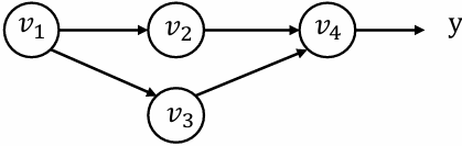
y can be written in the form of y = f(v₂,v₃)
$$
\overline{v}_1 = \frac{\partial y}{\partial v_1} = \frac{\partial f(v_2, v_3)}{\partial v_2} \frac{\partial v_2}{\partial v_1} + \frac{\partial f(v_2, v_3)}{\partial v_3} \frac{\partial v_3}{\partial v_1} = \overline{v}_2 \frac{\partial v_2}{\partial v_1} + \overline{v}3 \frac{\partial v_3}{\partial v_1}
$$
​ Define partial adjoint 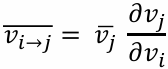for each input output node pair 𝑖 and 𝑗
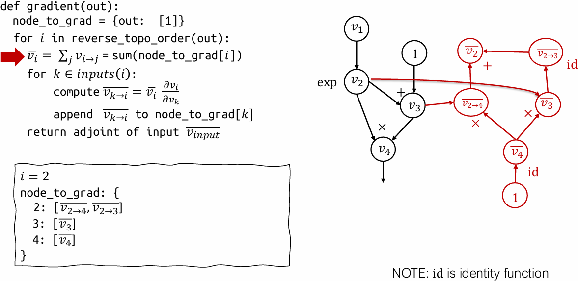
$$
\overline{v}i = \sum{j \in next(i)} \overline{v}{i \to j}
$$
​ We can compute partial adjoints separately then sum them together

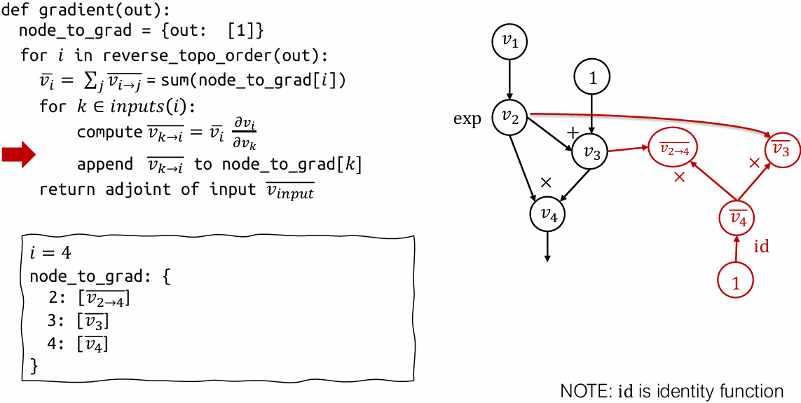
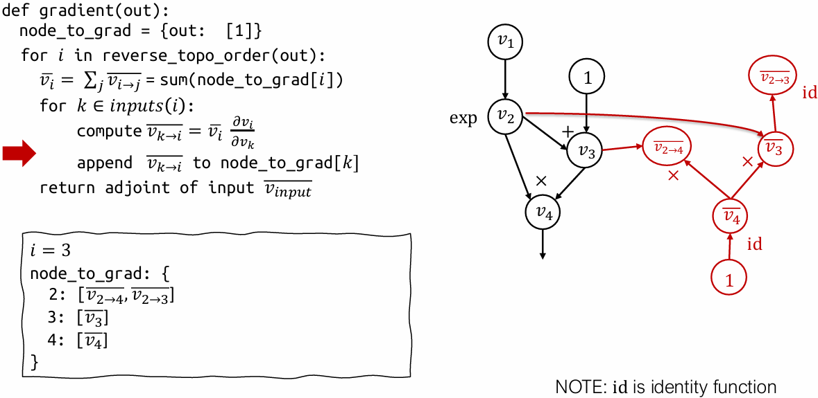
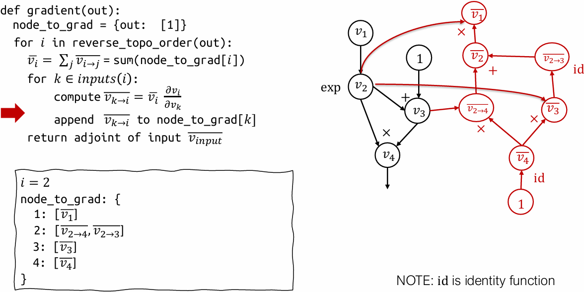
Reverse AD algorithm

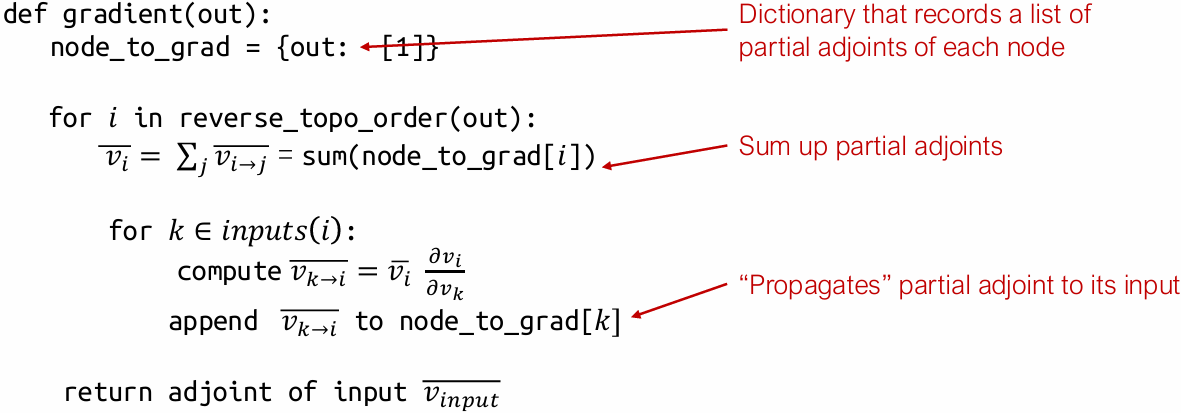
Reverse mode AD by extending computational graph
Our previous examples compute adjoint values directly by hand
How can we construct a computational graph that calculates the adjoint values?

Reverse mode AD vs Backprop
Backprop

Run backward operations the same forward graph
Used in first generation deep learning frameworks (caffe, cuda-convnet)
Reverse mode AD by extending computational graph

Construct separate graph nodes for adjoints
Used by modern deep learning frameworks

Reverse mode AD on Tensors

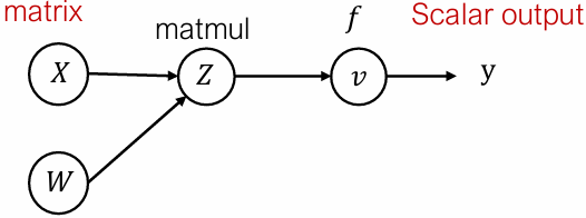
Define adjoint for tensor values
$$
\bar{Z} = \begin{bmatrix}
\frac{\partial y}{\partial Z_{1,1}} & \cdots & \frac{\partial y}{\partial Z_{1,n}} \
\vdots & \cdots & \vdots \
\frac{\partial y}{\partial Z_{m,1}} & \cdots & \frac{\partial y}{\partial Z_{m,n}}
\end{bmatrix}
$$
​ Forward evaluation trace
$$
\begin{align*}
Z_{ij} &= \sum_{k} X_{ik} W_{kj} \
v &= f(Z)
\end{align*}
$$
​ Forward matrix form
$$
\begin{align*}
Z &= XW \
v &= f(Z)
\end{align*}
$$
​ Reverse evaluation in scalar form
$$
\overline{X}{i,k} = \sum{j} \frac{\partial Z_{i,j}}{\partial X_{i,k}} \bar{Z}{i,j} = \sum{j} W_{k,j} \bar{Z}_{i,j}
$$
​ Reverse matrix form
$$
\bar{X} = \bar{Z} W^T
$$
Discussions
What are the pros/cons of backprop and reverse mode AD

Handling gradient of gradient
The result of reverse mode AD is still a computational graph
We can extend that graph further by composing more operations and run reverse mode AD again on the gradient
Part of homework 1

Reverse mode AD on data structures

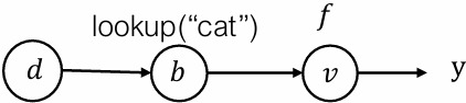
Define adjoint data structure
$$
\bar{d} = { \text{“cat”} : \frac{\partial y}{\partial a_0}, \text{“dog”} : \frac{\partial y}{\partial 1} }
$$
​ Forward evaluation trace
$$
\begin{align*}
d &= { \text{“cat”} : a_0, \text{“dog”} : a_1 } \
b &= d \text{ [“cat”]} \
v &= f(b)
\end{align*}
$$
​ Reverse evaluation
$$
\begin{align*}
\bar{b} &= \frac{\partial v}{\partial b} \bar{v} \
\bar{d} &= { \text{“cat”} : \bar{b} }
\end{align*}
$$
​ Key take away: Define “adjoint value” usually in the same data type as the forward value and adjoint propagation rule. Then the sample algorithm works
​ Do not need to support the general form in our framework, but we may support “tuple values”

Lecture 5: Automatic Differentiation Implementation

lecture5/5_automatic_differentiation_implementation.ipynb at main · dlsyscourse/lecture5

Lecture 6: Fully connected networks, optimization, initialization

Fully connected networks

Fully connected networks
Now that we have covered the basics of automatic differentiation, we can return to “standard” forms of deep networks
A L-layer, fully connected network, a.k.a. multi-layer perceptron (MLP), now with an explicit bias term, is defined by the iteration
$$
\begin{align*}
z_{i+1} &= \sigma_i(W_i^T z_i + b_i), \quad i = 1, \dots, L \
h_\theta(x) &\equiv z_{L+1} \
z_1 &\equiv x
\end{align*}
$$
​ with parameters θ = { W_1:L, b_1:L }, and where σ_i(x) is the nonlinear activation, usually with σ_L(x) = x

Matrix form and broadcasting subtleties
Let’s consider the matrix form of the the iteration
$$
Z_{i+1} = \sigma_i(Z_i W_i + \mathbf{1} b_i^T)
$$
​ Notice a subtle point: to write things correctly in matrix form, the update for Z_i+1 ∈ ℝ^m×n requires that we form the matrix 1b_i^T ∈ ℝ^m×n
​ In practice, you don’t form these matrices, you perform operation via broadcasting
​ E.g. for a n×1 vector (or higher-order tensor), broadcasting treats it as an nxp matrix repeating the same column p times
​ We could write iteration (informally) just as Z_i+1 = σ_i(Z_iW_i+b_i^T)
​ Broadcasting does not copy any data (described more in later lecture)

Key questions for fully connected networks
In order to actually train a fully-connected network (or any deep network), we need to address a certain number of questions:
How do we choose the width and depth of the network?
How do we actually optimize the objective? (“SGD” is the easy answer, but not the algorithm most commonly used in practice)
How do we initialize the weights of the network?
How do we ensure the network can continue to be trained easily over multiple optimization iterations?
All related questions that affect each other
There are (still) no definite answers to these questions, and for deep learning they wind up being problem-specific, but we will cover some basic principles

Optimization

Gradient descent
Let’s reconsider the generic gradient descent updates we described previously, now for a general function f, and writing iterate number t explicitly
$$
\theta_{t+1} = \theta_t - \alpha \nabla_\theta f(\theta_t)
$$
​ where α > 0 is step size (learning rate), 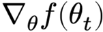is gradient evaluated at the parameters θ_t
​ Takes the “steepest descent direction” locally (defined in terms of ℓ₂ norm, as we will discuss shortly), but may oscillate over larger time scales

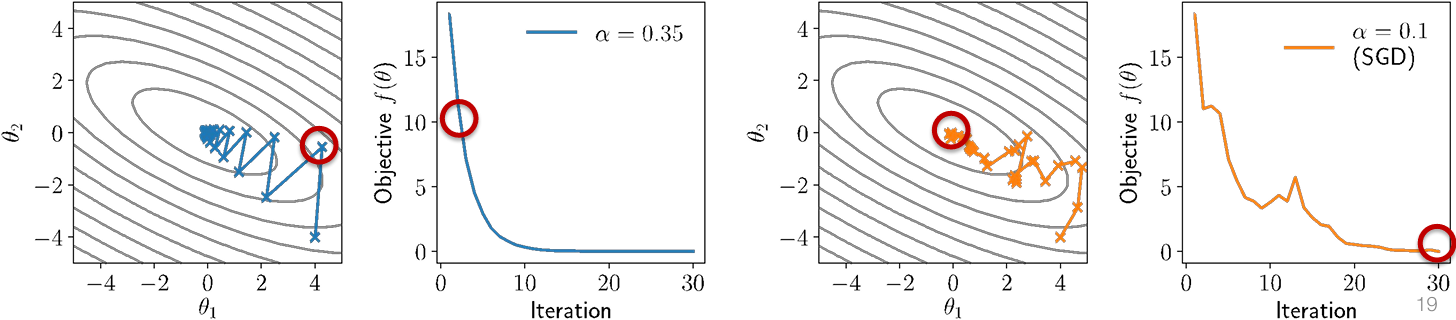
Illustration of gradient descent
For θ ∈ ℝ², consider quadratic function
$$
f(\theta) = \frac{1}{2} \theta^T P \theta + q^T \theta
$$
​ for P positive definite (all positive eigenvalues)
​ Illustration of gradient descent with different step sizes:

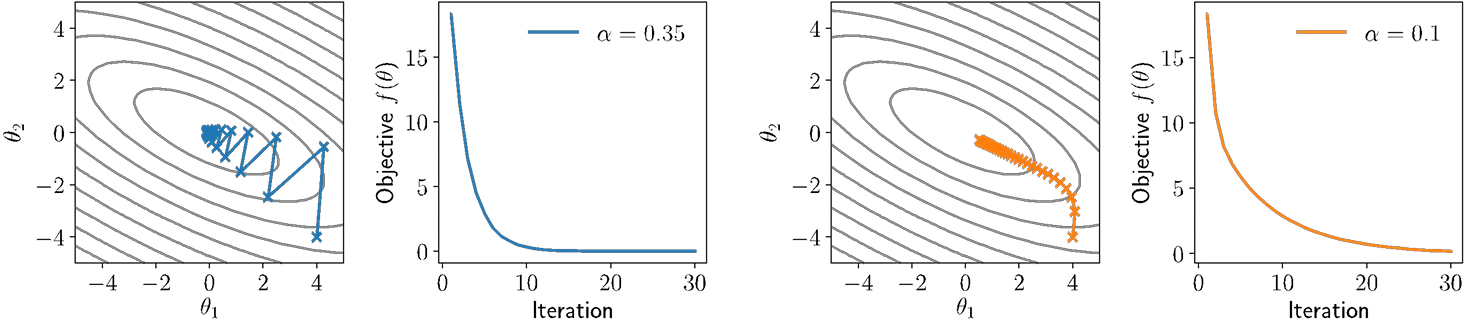
Newton’s Method
One way to integrate more “global” structure into optimization methods is Newton’s method, which scales gradient according to inverse of the Hessian (matrix of second derivatives)
$$
\theta_{t+1} = \theta_t - \alpha \left( \nabla^2_\theta f(\theta_t) \right)^{-1} \nabla_\theta f(\theta_t)
$$
​ where 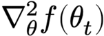is the Hessian, n×n matrix of all second derivatives
​ Equivalent to approximating the function as quadratic using second-order Taylor expansion, then solving for optimal solution
​ Full step given by α = 1, otherwise called a damped Newton method

Illustration of Newton’s method
Newton’s method (will α = 1) will optimize quadratic functions in one step
Not of that much practical relevance to deep learning for two reasons
We can’t efficiently solve for Newton step, even using automatic differentiation (though there are tricks to approximately solve it)
For non-convex optimization, it’s very unclear that we even want to use the Newton direction

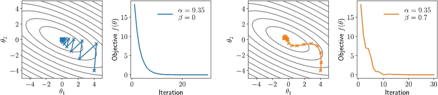
Momentum
Can we find “middle grounds” that are as easy to compute as gradient descent, but which take into account more “global” structure like Newton’s method
One common strategy is to use momentum update, that takes into account a moving average of multiple previous gradients
$$
\begin{aligned}
u_{t+1} &= \beta u_t + (1 - \beta) \nabla_\theta f(\theta_t) \
\theta_{t+1} &= \theta_t - \alpha u_{t+1}
\end{aligned}
$$
​ where α is step size as before, and β is momentum averaging parameter
​ Note: often written in alternative forms u_t+1 = βu_t + (or u_t+1 = βu_t + α) but I prefer above to keep u the same “scale” as gradient

Illustration of momentum
Momentum “smooths” out the descent steps, but can also introduce other forms of oscillation and non-descent behavior
Frequently useful in training deep networks in practice

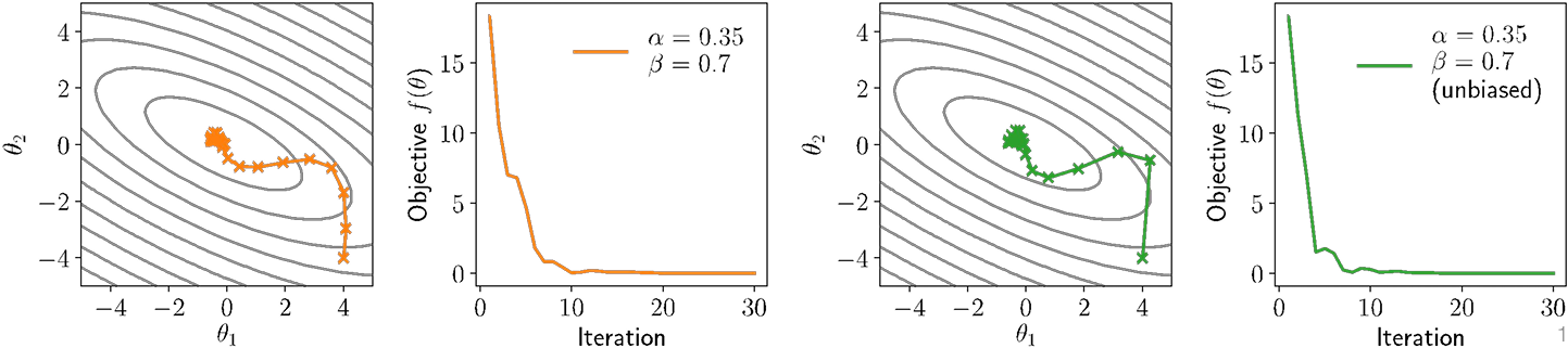
“Unbiasing” momentum terms
The momentum term u_t (if initialized to zero, as is common), will be smaller in initial iterations than in later ones
To “unbias” the update to have equal expected magnitude across all iterations, we can use the update
$$
\theta_{t+1} = \theta_t - \frac{\alpha u_{t+1}}{1 - \beta^{t+1}}
$$

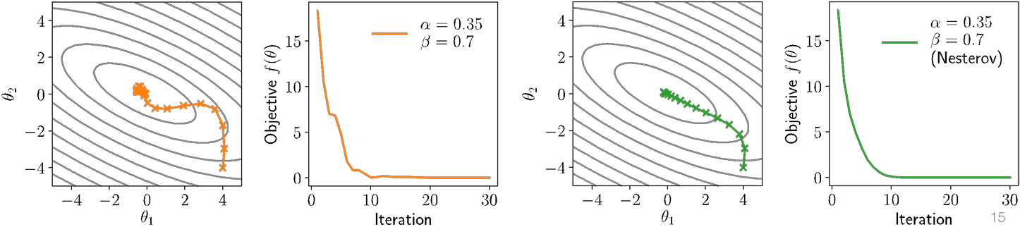
Nesterov Momentum
One (admittedly, of many) useful tricks in the notion of Nesterov momentum (or Nesterov acceleration), which computes momentum update at “next” point
$$
\begin{aligned}
u_{t+1} &= \beta u_t + (1 - \beta) \nabla_\theta f(\theta_t) \
\theta_{t+1} &= \theta_t - \alpha u_{t+1}
\end{aligned}
\quad \Longrightarrow \quad
\begin{aligned}
u_{t+1} &= \beta u_t + (1 - \beta) \nabla_\theta f(\theta_t - \alpha u_t) \
\theta_{t+1} &= \theta_t - \alpha u_{t+1}
\end{aligned}
$$
​ A “good” thing for convex optimization, and (sometimes) helps for deep networks

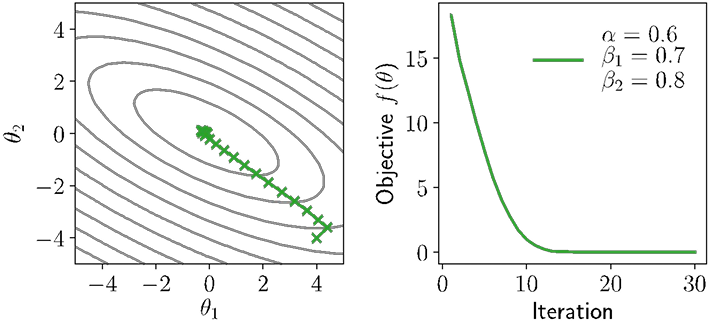
Adam
The scale of the gradients can vary widely for different parameters, especially e.g. across different layers of a deep network, different layer types, etc
So-called adaptive gradient methods attempt to estimate this scale over iterations and then re-scale the gradient update accordingly
Most widely used adaptive gradient method for deep learning is Adam algorithm, which combines momentum and adaptive scale estimation
$$
\begin{aligned}
u_{t+1} &= \beta_1 u_t + (1 - \beta_1) \nabla_\theta f(\theta_t) \
v_{t+1} &= \beta_2 v_t + (1 - \beta_2) \left( \nabla_\theta f(\theta_t) \right)^2 \
\theta_{t+1} &= \theta_t - \alpha \frac{u_{t+1}}{\sqrt{v_{t+1}} + \epsilon}
\end{aligned}
$$
​ (Common to use unbiased momentum estimated for both terms)

Notes on / illustration of Adam
Whether Adam is “good” optimizer is endlessly debated within deep learning, but it often seems to work quite well in practice (maybe?)
There are alternative universes where endless other variants became the “standard” (no unbiasing? average of absolute magnitude rather than squared? Nesterov-like acceleration?) but Adam is well-tuned and hard to uniformly beat

Stochastic variants
All the previous examples considered batch update to the parameters, but the single most important optimization choice is to use stochastic variants
Recall our machine learning optimization problem
$$
minimize_{\theta} \frac{1}{m} \sum_{i=1}^{m} \ell(h_\theta(x^{(i)}), y^{(i)})
$$
​ which is the minimization of an empirical expectation over losses
​ We can get a noisy (but unbiased) estimate of gradient by computing gradient of the loss over just a subset of examples (called a minibatch)

Stochastic Gradient Descent
This leads us again to the SGD algorithm, repeating for batches B ⊂ { 1, …, m }
$$
\theta_{t+1} = \theta_t - \frac{\alpha}{B} \sum_{i \in B} \nabla_\theta \ell(h(x^{(i)}), y^{(i)})
$$
​ Instead of taking a few expensive, noise-free, steps, we take many cheap, noisy steps, which ends having much strong performance per compute

The most important takeaways
All the optimization methods you have seen thus far presented are only actually used in their stochastic form
The amount of valid intuition about these optimization methods you will get from looking at simple (convex, quadratic) optimization problems is limited
You need to constantly experiment to gain an understanding / intuition of how these methods actually affect deep networks of different types

Initialization

Initialization of weights
Recall that we optimize parameters iteratively by stochastic gradient descent, e.g.
$$
W_i := W_i - \alpha \nabla_{W_i} \ell(h_\theta(X), y)
$$
​ But how do we choose the initial values of W_i, b_i? (maybe just initialize to zero?)
​ Recall the manual backpropagation forward/backward passes (without bias):
$$
Z_{i+1} = \sigma_i(Z_i W_i) \
G_i = \left( G_{i+1} \circ \sigma_i’(Z_i W_i) \right) W_i^\top \
\text{If } W_i = 0, \text{ then } G_j = 0 \text{ for } j \leq i \implies \nabla_{W_i} \ell(h_\theta(X), y) = 0 \
\text{i.e., } W_i = 0 \text{ is a (very bad) local optimum of the objective}
$$
Key idea #1: Weights don’t move “that much”
Might have the picture in your mind that the parameters of a network converge to some similar region of points regardless of their initialization
This is not true … weights often stay much closer to their initialization than to the “final” point after optimization from different
End result: initialization matters … we’ll see some of the practical aspects next lecture

Key idea #2: Choice of initialization matters
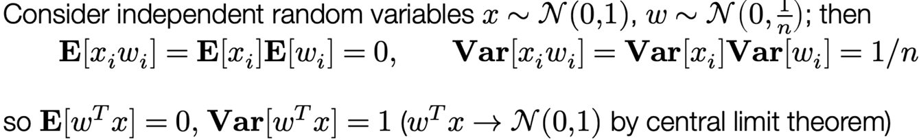
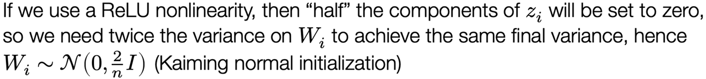
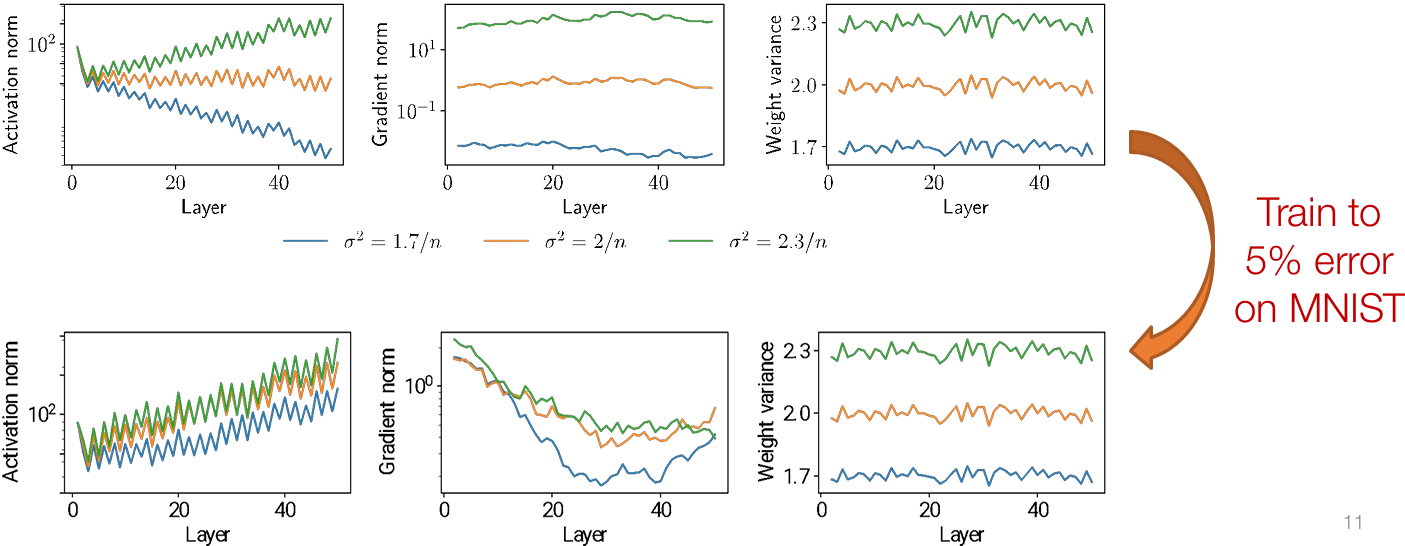
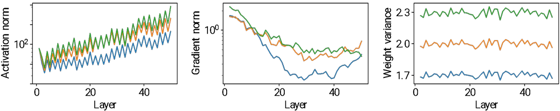
Let’s just initialize weights “randomly”, e.g., W_i ~ N(0, σ²I)
The choice of variance σ² will affect two (related) quantities:
The norm of the forward activations Z_i
The norm of the the gradients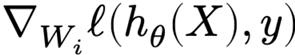
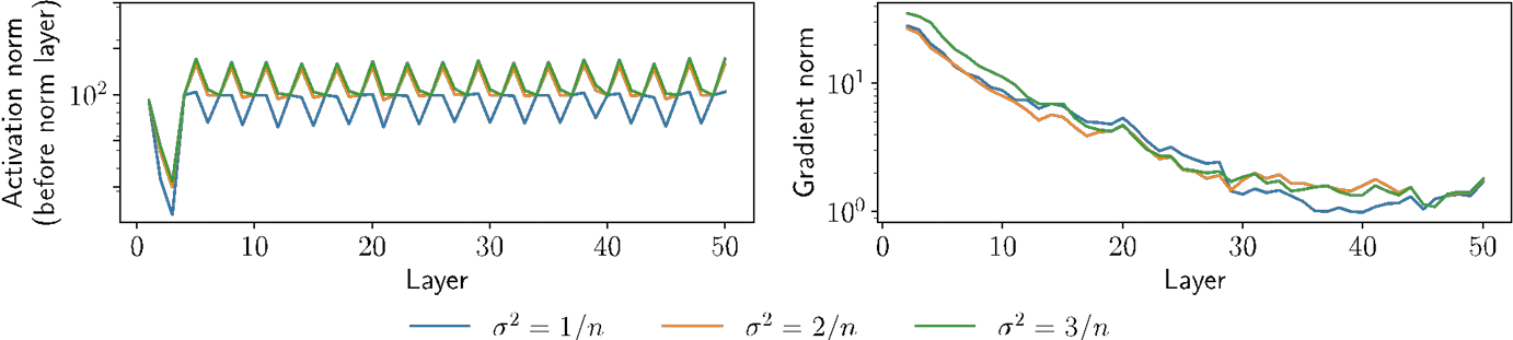
Illustration on MNIST with n = 100 hidden units, depth 50, ReLU nonlinearities

What causes these effects?

Homework 1

Lecture 7: Neural Network Library Abstractions

Programming abstractions

Programming abstractions
The programming abstraction of a framework defines the common ways to implement, extend and execute model computations
While the design choices may seem obvious after seeing them, it is useful to learn about the thought process, so that:
We know why the abstractions are designed in this way
Learn lessons to design new abstractions

Case studies

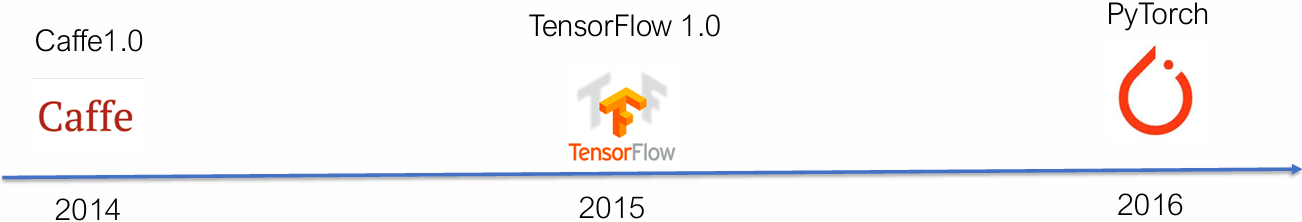
There are many frameworks being development along the way that we do not have time to study: theano, torch7, mxnet, caffe2, chainer, jax …

Forward and backward layer interface
Example framework: Caffe 1.0
Early pioneer: cuda-convnet

class Layer:
    def forward(bottom, top):
        pass
    def backward(top, propagate_down, bottom):
        pass

​ Defines the forward computation and backward(gradient) operations
​ Used in cuda-convenet (the AlexNet framework)

Computational graph and declarative programming
Example framework: Tensorflow 1.0
Early pioneer: Theano

import tensorflow as tf

v1 = tf.Variable()
v2 = tf.exp(v1)
v3 = v2 + 1
v4 = v2 * v3

sess = tf.Session()
value4 = sess.run(v4, feed_dict={v1: numpy.array([1])})

​ First declare the computational graph
​ Then execute the graph by feeding input value

Imperative automatic differentiation
Example framework: PyTorch (needle:)
Early pioneer: Chainer

import needle as ndl

v1 = ndl.Tensor([1])
v2 = ndl.exp(v1)
v3 = v2 + 1
v4 = v2 * v3

​ Executes computation as we construct the computational graph
​ Allow easy mixing of python control flow and construction

if v4.numpy() > 0.5:
    v5 = v4 * 2
else:
    v5 = v4
v5.backward()

Discussions
What are the pros and cons of each programming abstraction?

High level modular library components

Elements of Machine Learning
1.The hypothesis class:

2.The loss function:
$$
l(h_\theta(x), y) = -h_y(x) + \log \sum_{j=1}^k \exp(h_j(x))
$$
​ 3.An optimization method:
$$
\theta := \theta - \frac{\alpha}{B} \sum_{i=1}^{B} \left[ \nabla_{\theta} \ell(h_{\theta}(x^{(i)}), y^{(i)}) \right]
$$
​ Question: how do they translate to modular components in code?

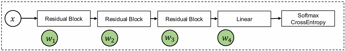
Deep learning is modular in nature
Deep learning is modular in nature

Residual block

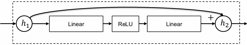
Linear

ReLU

Residual Connections
One of the most well-cited paper
Deep Residual Learning for Image Recognition | IEEE Conference Publication | IEEE Xplore
ResNetV2
Identity Mappings in Deep Residual Networks | Springer Nature Link

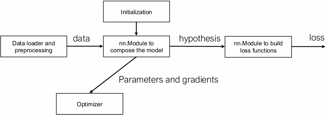
nn.Module: Compose Things Together
Residual block

Linear

Tensor in, tensor out
Key things to consider:
For given inputs, how to compute outputs
Get the list of (trainable) parameters
Ways to initialize the parameters

Loss functions as a special kind of module

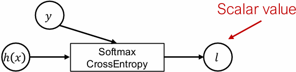
Tensor in, scalar out
$$
\ell(h_\theta(x), y) = -h_y(x) + \log \sum_{j=1}^{k} \exp\left(h_j(x)\right)
$$
​ Questions
​ How to compose multiple objective functions together?
​ What happens during inference time after training?

Optimizer
Model

Takes a list of weights from the model perform steps of optimization
Keep tracks of auxiliary states (momentum)
SGD
$$
w_i \leftarrow w_i - \alpha g_i
$$
​ SGD with momentum
$$
u_i \leftarrow \beta u_i + (1 - \beta) g_i \
w_i \leftarrow w_i - \alpha u_i
$$
​ Adam
$$
u_i \leftarrow \beta_1 u_i + (1 - \beta_1) g_i \
v_i \leftarrow \beta_2 v_i + (1 - \beta_2) g_i^2 \
w_i \leftarrow w_i - \alpha u_i / (v_i^{1/2} + \epsilon)
$$
Regularization and optimizer
Two ways to incorporate regularization:
Implement as part of loss function
Directly incorporate as part of optimizer update
SGD with weight decay (𝑙₂ regularization)
$$
w_i \leftarrow (1 - \alpha \lambda) w_i - \alpha g_i
$$
Initialization
Initialization strategy depends on the module being involved and the type of the parameter. Most neural network libraries have a set of common initialization routines
weights: uniform, order of magnitude depends on input/output
bias: zero
Running sum of variance: one
Initialization can be folded into the construction phase of a nn.module

Data loader and preprocessing
Data loading and augmentation pipeline

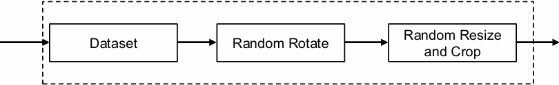
Model

We often preprocess (augment) the dataset by randomly shuffle and transform the input
Data augmentation can account for significant portion of prediction accuracy boost in deep learning models
Data loading and augmentation is also compositional in nature

Deep learning is modular in nature

Discussions
What are other possible examples of modular components?

Revisit programming abstraction
Example framework: Caffe 1.0

class Layer:
    def forward(bottom, top):
        pass
    def backward(top, propagate_down, bottom):
        pass

​ Couples gradient computation with the module composition

Revisit programming abstraction
Example framework: PyTorch (needle:)

import needle as ndl

v1 = ndl.Tensor([1])
v2 = ndl.exp(v1)
v3 = v2 + 1
v4 = v2 * v3

​ Two levels of abstractions
​ Computational graph abstraction on Tensors, handles AD
​ High level abstraction to handle modular composition

Lecture 8: Normalization and Regularization

Feature evolution

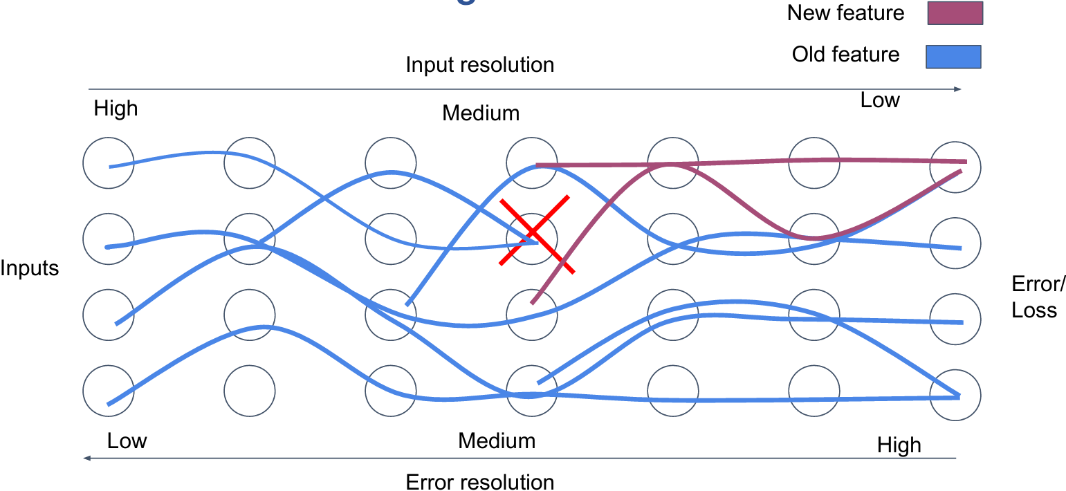
What are distributed feature representations?

How neural networks start to learn: Initial features

One initial feature for each class

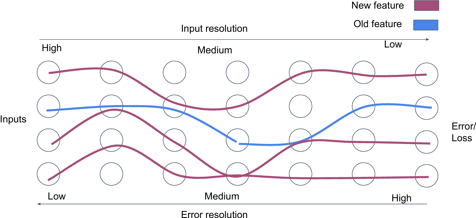
Overcoming feature competition

Normalization

Initialization vs. optimization
Suppose we choose W_i ~ N (0,c/n), where (for a ReLU network) c ≠ 2…
Won’t the the scale of the initial weights be “fixed” after a few iterations of optimization?
No! A deep network with poorly-chosen weights will never train (at least with vanilla SGD)


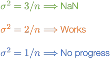
The problem is even more fundamental, however: even when trained successfully, the effects/scales present at initialization persist throughout training

Normalization
Initialization matters a lot for training, and can vary over the course of training to no longer be “consistent” across layers / networks
But remember that a “layer” in deep networks can be any computation at all…
…let’s just add layers that “fix” the normalization of the activations to be whatever we want!

Batch and layer normalization

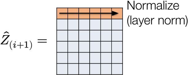
Layer normalization
First idea: let’s normalize (mean zero and variance one) activations at each layer; this is known as layer normalization
$$
\begin{aligned}
\hat{z}{i+1} &= \sigma_i(W_i^T z_i + b_i) \
z{i+1} &= \frac{\hat{z}{i+1} - \mathbb{E}[\hat{z}{i+1}]}{(\text{Var}[\hat{z}_{i+1}] + \epsilon)^{1/2}}
\end{aligned}
$$
​ Also common to add an additional scalar weight and bias to each term (only changes representation e.g., if we put normalization prior to nonlinearity instead)

LayerNorm illustration
“Fixes” the problem of varying norms of layer activations (obviously)

In practice, for standard FCN, harder to train resulting networks to low loss (relative norms of examples are a useful discriminative feature)

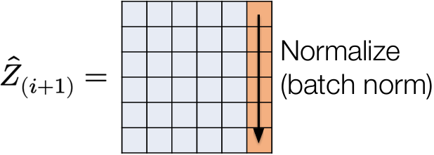
Batch normalization
An odd idea: let’s consider the matrix form of our updates
$$
\hat{Z}_{i+1} = \sigma_i(Z_i W_i + b_i^T)
$$
​ then layer normalization is equivalent to normalizing the rows of this matrix
​ What if, instead, we normalize it’s columns? This is called batch normalization, as we are normalizing the activations over the minibatch
​

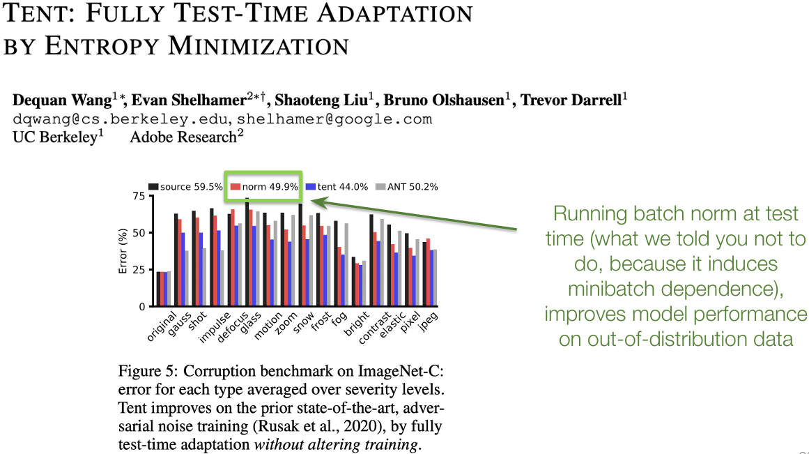
Minibatch dependence
One oddity to BatchNorm is that it makes the predictions for each example dependent on the entire batch
Common solution is to compute a running average of mean/variance for all features at each layer 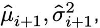and at test time normalize by these quantities
$$
(z_{i+1})j = \frac{(\hat{z}{i+1})j - (\hat{\mu}{i+1})j}{\left( (\hat{\sigma}^2{i+1})_j + \epsilon \right)^{1/2}}
$$

Regularization

Regularization of deep networks
Typically deep networks (even the simple two layer network you wrote in the homework) are overparameterized models: they contain more parameters (weights) than the number of training examples
This means (formally, under a few assumptions), that they are capable of fitting the training data exactly
In “traditional” ML/statistical thinking (with a number of big caveats), this should imply that the models will overfit the training set, and not generalize well
… but they do generalize well to test examples
… but not always (many larger models will often still overfit)

Regularization
Regularization is the process of “limiting the complexity of the function class” in order to ensure that networks will generalize better to new data; typically occurs in two ways in deep learning
Implicit regularization refers to the manner in which our existing algorithms (namely SGD) or architectures already limit functions considered
E.g., we aren’t actually optimizing over “all neural networks”, we are optimizing over all neural networks considered by SGD, with a given weight initialization
Explicit regularization refers to modifications made to the network and training procedure explicitly intended to regularize the network

ℓ₂ Regularization a.k.a. weight decay
Classically, the magnitude of a model’s parameters are often a reasonable proxy for complexity, so we can minimize loss while also keeping parameters small
$$
minimize_{W_{1:L}} \frac{1}{m} \sum_{i=1}^{m} \ell\big( h_{W_{1:L}}(x^{(i)}), y^{(i)} \big) + \frac{\lambda}{2} \sum_{i=1}^{L} | W_i |2^2
$$
​ Results in the gradient descent updates:
$$
W_i := W_i - \alpha \nabla{W_i} \ell(h(X), y) - \alpha \lambda W_i = (1 - \alpha \lambda) W_i - \alpha \nabla_{W_i} \ell(h(X), y)
$$
​ I.e., at each iteration we shrink the weights by a factor (1 – αλ) before taking the gradient step

Caveats of ℓ₂ regularization
ℓ₂ regularization is exceedingly common deep learning, often just rolled into the optimization procedure as a “weight decay” term
However, recall our optimized networks with different initializations:

… Parameter magnitude may be a bad proxy for complexity in deep networks

Dropout
Another common regularization strategy: randomly set some fraction of the activations at each layer to zero
$$
\begin{aligned}
\hat{z}{i+1} &= \sigma_i(W_i^T z_i + b_i) \
(z{i+1})j &=
\begin{cases}
(\hat{z}{i+1})_j / (1 - p) & \text{with probability } 1 - p \
0 & \text{with probability } p
\end{cases}
\end{aligned}
$$
​ (Not unlike BatchNorm) seems very odd on first glance: doesn’t this massively change the function being approximated?

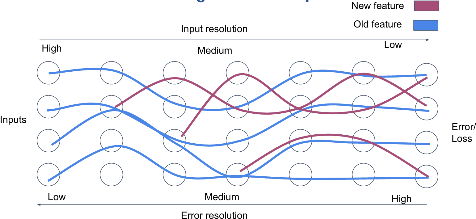
Overcoming feature saturation

Interaction of optimization, initialization, normalization, regularization

Many solutions … many more questions
Many design choices meant to ease optimization ability of deep networks
Choice of optimizer learning rate / momentum
Choice of weight initialization
Normalization layer
Reguarlization
These factors all (of course) interact with each other
And these don’t even include many other “tricks” we’ll cover in later lectures: residual connections, learning rate schedules, others I’m likely forgetting
…you would be forgiven for feeling like the practice of deep learning is all about flailing around randomly with lots of GPUs

BatchNorm: An illustrative example

​ “Here is what we know about batch norm as a field. It works because it reduces internal covariant shift. Wouldn’t you like to know why reducing internal covariant shift speeds up gradient descent? Wouldn’t you like to see a theorem or an experiment? Wouldn’t you like to know, wouldn’t you like to see evidence that batch norm reduces internal covariant shift? Wouldn’t you like to know what internal covariant shift is? Wouldn’t you like to see a definition of it?” - Ali Rahimi (NeurIPS 2017 Test of Time Talk)

​

​

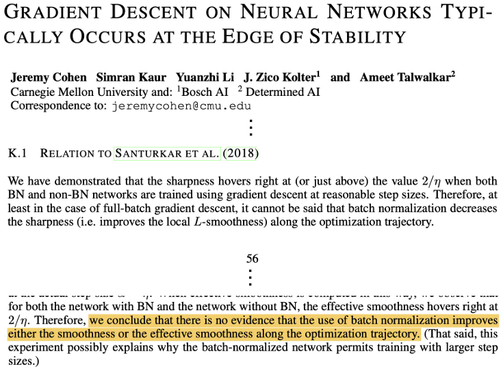
BatchNorm: Other benefits?

The ultimate takeaway message
I don’t want to give the impression that deep learning is all about random hacks: there have been a lot of excellent scientific experimentation with all the above
But it is true that we don’t have a complete picture of how all the different empirical tricks people use really work and interact
The “good” news is that in many cases, it seems to be possible to get similarly good results with wildly different architectural and methodological choices

Lecture 9: NN Library Implementation

lecture8/8_nn_library_implementation.ipynb at main · dlsyscourse/lecture8

Lecture 10:

Homework 2